⚖️ The trade-off: privacy, performance, and price
Nothing is truly free—you always trade one thing for another. Local gives you privacy and zero cost, but you pay in raw performance. In this module, you’ll learn to READ this trade-off critically: what each dimension gains, what it loses, and why “1 year behind the frontier” is already more than enough for most of your work.
🔐 Privacy: what you gain
Let's start with the area where local wins by a mile: privacy. When the model runs on your machine, the text you type, the files you open, and the answers you receive never leave there. There’s no third-party server in the middle, no company keeping a record, and no retention policy that could change tomorrow. The data is yours and stays yours.
🛡️ The three “never” rules for local use
- •The data never travels over the internet — it sits between the keyboard and the disk.
- •No company never stores what you ask to train another model.
- •Access never depends on a login that can be revoked.
New here? "Trade-off" means improving one thing at the expense of another—there’s no free lunch. The central trade-off here is that you gain privacy and lower costs in exchange for giving up a little raw performance. The whole module is about measuring that trade-off honestly.
Key concepts
Every choice improves one axis and costs you another; the secret is choosing deliberately.
The data can't leave because there's NO way out, not because someone promises it won't.
No logs are stored on a server you don’t control.
No one cuts off your access to your own model.
⚡ Performance: the "1 year behind" frontier
Now the dimension where local falls behind—but by less than you might think. The best open models that run on your laptop today are, on average, about a year behind the frontier (the leading cloud models). The good news: today's frontier is astonishingly good, so "a year ago" is still excellent for the vast majority of everyday tasks.
Notice: the model today’s local is at the level where the frontier was a year ago. Since the frontier model from a year ago was already great, today's local model handles almost everything — and the gap stays constant instead of exploding.
✓ Where "1 year behind" is enough
- ✓Summarize, rewrite, translate, and reply to email.
- ✓Draft code and explain snippets.
- ✓Chat about private documents.
- ✓Repetitive tasks running all day.
✗ Where the boundary still wins
- ✗Very long and difficult reasoning problems.
- ✗Large, complex coding tasks (see benchmarks).
- ✗When that last 5% of quality changes the result.
- ✗When cloud speed matters more than privacy.
Key concepts
The top models of the moment, almost always running in the cloud.
The typical lag between the best open model and the frontier.
For most tasks, “1 year ago” is more than recent enough.
Open models improve alongside the frontier; the gap doesn’t grow.
💰 Price: $0 per use, forever
The third axis: price. In the cloud, you pay per token — every question and every answer has a meter running. Locally, after downloading the model just once, each use is free. There's no bill at the end of the month, no "you spent X dollars today." The only cost is the hardware you already have and a little electricity.
📊 Cost: cloud vs. local
- •Cloud: VARIABLE cost that rises with usage (OPEX) — the more you use it, the more you pay.
- •Local: FIXED cost already paid (the computer) + ~$0 per call (CAPEX).
- •Since each call costs $0, you can leave 24/7 agents without worrying about the bill — that’s the topic of 1.6.
💡 Practical tip
Since exploring is free, download, test, and delete models as much as you like. The "price" of getting it wrong is zero. Treat each download as a cheap experiment, not a commitment.
Key concepts
Free to use after download — no meter.
Invest in hardware once instead of paying for recurring usage.
Predictable cost: you already know it’s zero.
The only paid “usage” is the electricity for your machine.
📊 Benchmarks: read them critically
Here, the trade-off becomes number. The chart below is the SWE-bench — a test of solving real programming problems. The score is the percentage of tasks the model solves on its own. The higher, the better. It’s worth reading carefully: the frontier leads, but the model that “runs on a laptop” comes close enough to impress.
New here? "Benchmark" is a standardized test for comparing models using the same yardstick. "SWE-bench" measures the ability to solve real software bugs and tasks. The number is the percentage of tasks solved—don’t confuse it with a "test score"; it’s difficult, and even the frontier models don’t reach 90%.
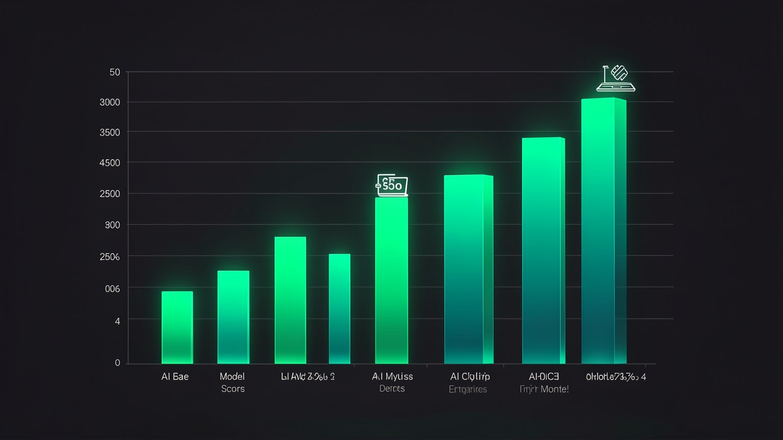
🔢 The actual numbers (SWE-bench, from the video)
The critical reading: o Qwen 3.6 27B, marked as "runs on a laptop", it does 74.0 — against 88.6 of Opus 4.8 in the cloud. That’s ~14.6 points of difference for a model that fits on your machine, runs offline, and costs $0 per use. That’s exactly the "1 year behind" thesis: close enough for almost everything.
Key concepts
Test of solving real software tasks; % of tasks solved.
Frontier (Opus 4.8) vs. local (Qwen 3.6 27B): ~14.6 points.
Qwen 74.0 fits on your machine—nearly half the list.
14 points on paper rarely translate into 14 points in YOUR work.
🐢 As fast as your machine
There’s a fourth hidden axis in “performance”: speed. In the cloud, you rent massive GPUs, so the response is fast no matter what computer you have. Locally, the speed depends entirely on your your hardware — chip, memory, and model size. A larger model on a modest machine will respond slowly; the same model on a powerful chip flies.
The chip sets the pace
A modern chip (e.g., an Apple M with plenty of unified memory) generates tokens much faster.
Larger model = slower
More parameters mean more weight; a smaller model responds faster on the same machine.
The choice is yours
You strike a balance: a smaller, faster model for everyday tasks and a larger, more capable model for the heavy lifting.
Practical tip: local speed isn’t fixed — it’s adjustable. If a model is slow, switch to a smaller or more heavily quantized one (we’ll cover this in Track 2). “Slow” almost always means “the model is too large for this hardware,” not “local is bad.”
Key concepts
Local speed depends on YOUR chip and memory, not a server.
A larger model responds more slowly on the same machine.
On Apple M chips, RAM and GPU share memory — a big help.
Switching models changes the speed — “slow” can be fixed.
🧩 Divide the work into percentages
The practical takeaway from the trade-off: you doesn't pick a side. You divide the work. Imagine that 100% of your tasks use AI. One portion requires absolute privacy — use local. Another requires the best possible answer — use frontier. Another just needs to be fast and cheap — local again. Each portion has the right tool, and the secret is to route deliberately.
The entire bar is your work. The most comes down to local (privacy, cost, everyday use); the frontier slice comes in only when that last 5% of quality changes the result. Planning those slices is what Hermes does with the three modes.
🧭 Bridge to the next module
This percentage breakdown isn’t just theoretical. In the module 1.6 it becomes the three concrete Hermes modes— Vault (all local), Connected (middle ground) and Cloud (maximum quality). You'll learn when to use each one.
In Track 3, you'll build a workflow that switches between them based on how sensitive the task is.
Key concepts
Each slice of the work calls for the right tool—don’t pick just one side.
Send each task to the right place, intentionally.
The cloud comes in only when that last 5% of quality matters.
Vault, Connected, and Cloud — the topic of module 1.6.
Optional self-check: In the video’s SWE-bench, what’s the honest take on Qwen 3.6 27B "runs on a laptop"?
🎯 Module summary
Next module:
1.6 — The three modes: Vault, Connected, and Cloud